![]()
This article covers:
- One-dimensional and two-dimensional NumPy arrays
- Generating NumPy arrays randomly
- Operations with NumPy arrays: element-wise operations, summarizing operations, sorting and filtering
To go through this tutorial, you need to have Python and Jupyter Notebook. The easiest way to get them is to use Anaconda.
For a Python refresher, check Introduction to Python.
NumPy
NumPy is a short name for “Numerical Python” – it’s a Python library for numerical manipulations. NumPy plays a central role in the python machine learning ecosystem: nearly all the libraries in Python depend on it. For example, Pandas, Scikit-Learn, and TensorFlow all rely on NumPy for numerical operations.
NumPy comes pre-installed in Anaconda distribution of NumPy, so if you use it, you don’t need to do anything extra. But if you don’t use Anaconda, installing NumPy is quite simple with pip:
pip install numpy
In order to use NumPy, we need to import it. That’s why in the first cell we write the import:
import numpy as np
In the scientific Python community, it’s common to use an alias when importing NumPy, that’s why we add “as np” in the code. This allows us to write “np” in the code instead of “numpy”.
We’ll start exploring NumPy from its core data structure: NumPy array.
NumPy arrays
NumPy arrays are similar to Python lists, but they are better optimized for number crunching tasks – like machine learning.
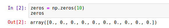
To create an array of a predefined size filled with zeros, we use the np.zeros function:
zeros = np.zeros(10)
This creates an array with ten zero elements:
Likewise, we can create an array with ones using the np.ones function:
ones = np.ones(10)
It works exactly in the same way as zeros, except the elements are ones.
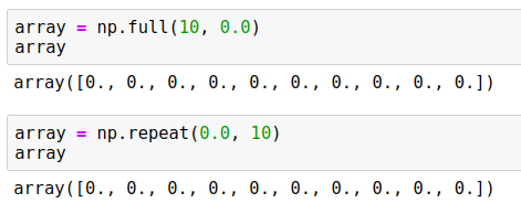
Both functions are a shortcut for a more general function np.full: it creates an array of a certain size filled with the specified element. For example, to create an array of size 10 filled with zeros, we do the following:
array = np.full(10, 0.0)
We can achieve the same result using the np.repeat function:
array = np.repeat(0.0, 10)
This code produces the same result as the code above:
While in this example both functions produce the same code, np.repeat is actually more powerful. For example, we can use it to create an array where multiple elements are repeated one after another:
array = np.repeat([0.0, 1.0], 5)
It creates an array of size 10 where the number 0 is repeated 5 times, and then the number 1 is repeated 5 times:
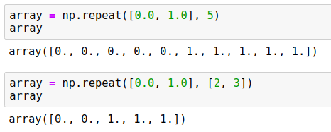
We can even be more flexible and specify how many times each element should be repeated:
array = np.repeat([0.0, 1.0], [2, 3])
In this case, 0.0 is repeated 2 times and 1.0 is repeated 3 times:
array([0., 0., 1., 1., 1.])
Like with lists, we can access an element of an array with square brackets:
el = array[1]
print(el)
This code prints “0.0”.
Unlike usual Python lists, we can access multiple elements of the array at the same time by using a list with indices in the square brackets:
print(array[[4, 2, 0]])
The result is another array of size 3 consisting of elements of the original array indexed by 4, 2 and 0 respectively:
[1., 1., 0.]
We can also update the elements of the array using square brackets:
array[1] = 1
print(array)
Since we changed the element at index 1 from “0” to “1”, it prints the following:
[0. 1. 1. 1. 1.]
If we already have a list with numbers, we can convert it to a NumPy array using np.array:
elements = [1, 2, 3, 4]
array = np.array(elements)
Now array is a NumPy array of size 4 with the same elements as the original list:
array([1, 2, 3, 4])
Another useful function for creating NumPy arrays is np.arange: it’s the NumPy equivalent of Python’s range:
np.arange(10)
It creates an array of length 10 with numbers from 0 to 9, and like in standards Python’s range, 10 is not included in the array:
array([0, 1, 2, 3, 4, 5, 6, 7, 8, 9])
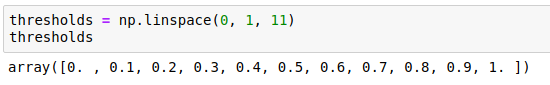
Often we need to create an array of a certain size filled with numbers between some number x and some number y. For example, imagine that we need to create an array with number from 0 to 1:
We can use np.linspace for doing it:
thresholds = np.linspace(0, 1, 11)
This function takes three parameters:
- The starting number – in our case, we want to start from 0
- The last number – we want to finish with 1
- The length of the resulting array – in our case, we want 11 numbers in the array.
This code produces 11 numbers from 0 till 1:
Usual Python lists can contain elements of any type. This is not the case for NumPy arrays: all elements of an array must have the same type. These types are called dtypes.
There are four broad categories of dtypes:
- Unsigned integers (
uint) – integers that are always positive (or zero) - Signed integers (
int) – integers that can be positive and negative - Floats (
float) – real numbers - Booleans (
bool) – only True and False values
There are multiple variations of each dtype depending on the number of bits used for representing the value in memory.
For uint we have four types: uint8, uint16, uint32, uint64 of size 8, 16, 32 and 64 bits respectively. Likewise, we have four types of int: int8, int16, int32 and int64. The more bits we use, the larger numbers we can store:
| Size (bits) | uint | int | float |
| 8 | 0 .. 28 - 1 | -27 .. 27 - 1 | - |
| 16 | 0 .. 216 - 1 | -215 .. 215 - 1 | Half precision |
| 32 | 0 .. 232 - 1 | -231 .. 231 - 1 | Single precision |
| 64 | 0 .. 264 - 1 | -263 .. 263 - 1 | Double precision |
In the case of floats, we have three types: float16, float32, and float64. The more bits we use, the more precise the float is. For most machine learning applications, float32 is good enough: we typically don’t need great precision.
You can check the full list of different dtypes in the official documentation.
Note: In NumPy, the default float dtype is
float64, which uses 64 bits (8 bytes) for each number. For most machine learning applications we don’t need such precision and we can reduce the memory footprint two times by usingfloat32instead offloat64.
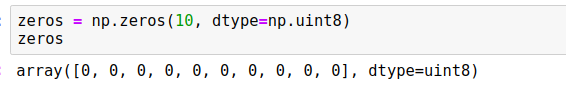
When creating an array, we can specify the dtype. For example, when using np.zeros and np.ones, the default dtype is float64. We can specify the dtype when creating an array:
zeros = np.zeros(10, dtype=np.uint8)
When we have an array with integers and assign a number outside of the range, the number is cut: only the least significant bits are kept.
For example, suppose we use the uint8 array zeros we just created. Since the dtype is uint8, the largest number it can store is 255. Let’s try to assign 300 to the first element of the array:
zeros[0] = 300
print(zeros[0])
Since 300 is greater than 255, only the least significant bits are kept, so this code prints “44”.
Warning: Be careful when choosing the dtype for an array. If you accidentally choose a dtype that’s too narrow, NumPy won’t warn you when you put in a big number. It will simply truncate them.
Iterating over all elements of an array is similar to list: we simply can use a for loop:
for i in np.arange(5):
    print(i)
This code prints numbers from 0 till 4:
0
1
2
3
4
Two-dimensional NumPy arrays
So far we have covered one-dimensional NumPy arrays. We can think of these arrays as vectors. However, for machine learning applications, having only vectors is not enough: we also often need matrices.
In plain Python, we’d use a list of lists for that. In NumPy, the equivalent is a two-dimensional array.
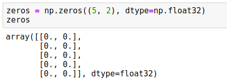
To create a two-dimensional arrays with zeros, we simply use a tuple instead of a number when invoking np.zeros:
zeros = np.zeros((5, 2), dtype=np.float32)
We use a tuple “(5, 2)”, so it creates an array of zeros with 5 rows and 2 columns:
In the same way, we can use np.ones or np.fill – instead of a single number, we put in a tuple.
The dimensionality of an array is called shape. This is the first parameter we pass to the np.zeros function: it specifies how many rows and columns the array will have. To get the shape of an array, use the shape property:
print(zeros.shape)
When we execute it, we see “(5, 2)”.
It’s possible to convert a list of lists to a NumPy array. Like with usual lists of numbers, simply use np.array for that:
numbers = [
    [1, 2, 3],
    [4, 5, 6],
    [7, 8, 9]
]

numbers = np.array(numbers)
After executing this code, numbers becomes a NumPy array with shape (3, 3). When we print it, we get:
array([[1, 2, 3],
       [4, 5, 6],
       [7, 8, 9]])
To access an element of a two-dimensional array, we need to use two numbers inside the brackets:
print(numbers[0, 1])
This code will access the row indexed by 0 and column indexed by 1. So it will print “2”.
Like with one-dimensional arrays, we use the assignment operator (“=”) to change an individual value of a two-dimensional array:
numbers[0, 1] = 10
When we execute it, the content of the array changes:
array([[ 1, 10,  3],
       [ 4,  5,  6],
       [ 7,  8,  9]])
If instead of two numbers, we put only one, we get the entire row, which is a one-dimensional NumPy array:
numbers[0]
This code returns the entire row indexed by 0:
array([1 2 3])
To access a column of a two-dimensional array, we use a colon (“:”) instead of the first element. Like with rows, the result is also a one-dimensional NumPy array:
numbers[:, 1]
When we execute it, we see the entire column:
array([2 5 8])
It’s also possible to overwrite the content of the entire row or a column using the assignment operator. For example, suppose we want to replace a row in the matrix:
numbers[1] = [1, 1, 1]
This results in the following change:
array([[ 1, 10,  3],
       [ 1,  1,  1],
       [ 7,  8,  9]])
Likewise, we can replace the content of an entire column:
numbers[:, 2] = [9, 9, 9]
As a result, the last column changes:
array([[ 1, 10,  9],
       [ 1,  1,  9],
       [ 7,  8,  9]])
Randomly generated arrays
Often it’s useful to generate arrays filled with random numbers. To do it in NumPy, we use the np.random module.
For example, to generate a 5x2 array of random numbers uniformly distributed between 0 and 1, use np.random.rand:
arr = np.random.rand(5, 2)
When we run it, it generates an array that looks like that:
array([[0.64814431, 0.51283823],
       [0.40306102, 0.59236807],
       [0.94772704, 0.05777113],
       [0.32034757, 0.15150334],
       [0.10377917, 0.68786012]])
Every time we run the code, it generates a different result. Sometimes we need the results to be reproducible, which means that if we want to execute this code later, we will get the same results. To achieve that, we can set the seed of the random number generator. Once the seed is set, the random number generator produces the same sequence every time we run the code.
np.random.seed(2)
arr = np.random.rand(5, 2)
On Ubuntu Linux 18.04 with NumPy version 1.17.2 it generates the following array:
array([[0.4359949 , 0.02592623],
       [0.54966248, 0.43532239],
       [0.4203678 , 0.33033482],
       [0.20464863, 0.61927097],
       [0.29965467, 0.26682728]])
No matter how many times we re-execute this cell, the results are the same.
Warning: Fixing the seed of the random number generator guarantees that the generator will produce the same results when executed on the same OS with the same NumPy version. However, there’s no guarantee that updating the NumPy version will not affect reproducibility: a change of version may result in changes in the random number generator algorithm, and that may lead to different results across versions.
If instead of uniform distribution, we want to sample from the standard normal distribution, we use np.random.randn:
arr = np.random.randn(5, 2)
Note: Every time we generate a random array in this article, we fix the seed number (we use “2”), even if we don’t explicitly specify it in the code.
To generate uniformly distributed random integers between 0 and 100 (exclusive), we can use np.random.randint:
randint = np.random.randint(low=0, high=100, size=(5, 2))
When executing the code, we get a 5x2 NumPy array of integers:
array([[40, 15],
       [72, 22],
       [43, 82],
       [75,  7],
       [34, 49]])
Another quite useful feature is shuffling an array – rearranging the elements of an array in random order. For example, let’s create an array with a range and then shuffle it:
idx = np.arange(5)
print('before shuffle', idx)

np.random.shuffle(idx)
print('after shuffle', idx)
When we run the code, we see the following:
before shuffle [0 1 2 3 4]
after shuffle  [2 3 0 4 1]
NumPy operations
NumPy comes with a wide range of operations that work with the NumPy arrays. In this section we’ll cover operations that we’ll need throughout the book.
Element-wise operations
NumPy arrays support all the arithmetic operations: addition (“+”), subtraction (“-”), multiplication (“*”), division (“/”) and others.
To illustrate these operations, let’s first create an array using arange:
rng = np.arange(5)
This array contains five elements from 0 till 4:
array([0, 1, 2, 3, 4])
To multiply every element of the array by two, we simply use the multiplication operator (“*”):
rng * 2
As a result, we get a new array where each element from the original array is multiplied by two:
array([0, 2, 4, 6, 8])
We don’t need to explicitly write any loops here to apply the multiplication operation individually to each element: NumPy does it for us. We can say that the multiplication operation is applied element-wise – to all elements at once. The addition (“+”), subtraction (“-”) and division (“/”) operations are also element-wise and require no explicit loops.
Such element-wise operations are often called vectorized: the for loop happens internally in native code (written C and fortran), so the operations are very fast!
Note: Whenever possible, use vectorized operations from NumPy instead of loops: they are always a magnitude faster.
In the previous code we used only one operation. It’s possible to apply multiple operations at once in one expression:
(rng - 1) * 3 / 2 + 1
This code creates a new array with the result:
array([-0.5, 1. , 2.5, 4. , 5.5])
The original array contains integers, but because we used the division operation, the result is an array with float numbers.
Previously, our code involved an array and simple Python numbers. It’s also possible to do element-wise operations with two arrays – if they have the same shape.
For example, suppose we have two arrays, one containing numbers from 0 to 4, and another containing some random noise:
noise = 0.01 * np.random.rand(5)
numbers = np.arange(5)
We sometimes need to do that for modeling not-ideal real-life data: in reality there are always imperfections when the data is collected, and we can model these imperfections by adding noise.
We build the noise array by first generating numbers between 0 and 1 and then multiplying them by 0.01. This effectively generates random numbers between 0 and 0.01:
array([0.00435995, 0.00025926, 0.00549662, 0.00435322, 0.00420368])
We can then add these two arrays and get a third one with the sum:
result = numbers + noise
In this array, each element of the result is the sum of the respective elements of the two other arrays:
array([0.00435995, 1.00025926, 2.00549662, 3.00435322, 4.00420368])
We can round the numbers to any precision using the round method:
result.round(4)
It’s also an element-wise operation, so it’s applied to all the elements at once and the numbers are rounded to the 4th digit:
array([0.0044, 1.0003, 2.0055, 3.0044, 4.0042])
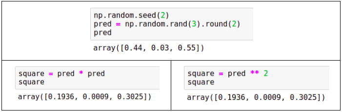
Sometimes we need to square all the elements of an array. For that, we can simply multiply the array with itself. Let’s first generate an array:
pred = np.random.rand(3).round(2)
This array contains 3 random numbers:
array([0.44, 0.03, 0.55])
Now we can multiply it with itself:
square = pred * pred
As a result, we get a new array where each element of the original array is squared:
array([0.1936, 0.0009, 0.3025])
Alternatively, we can use the power operator (“**”):
square = pred ** 2
Both approaches lead to the same results
Other useful element-wise operations that we might need for machine learning applications are exponent, logarithm and square root:
pred_exp = np.exp(pred) # exponent
pred_log = np.log(pred) # logarithm
pred_sqrt = np.sqrt(pred) # square root
Boolean operations can also be applied to NumPy arrays element-wise. To illustrate them, let’s again generate an array with some random numbers:
pred = np.random.rand(3).round(2)
This array contains the following numbers:
array([0.44, 0.03, 0.55])
We can see what the elements that are greater than 0.5:
result = predictions >= 0.5
As a result, we get an array with three boolean values:
array([False, False, True])
We know that only the last element of the original array is greater than 0.5, so it’s True and the rest are False.
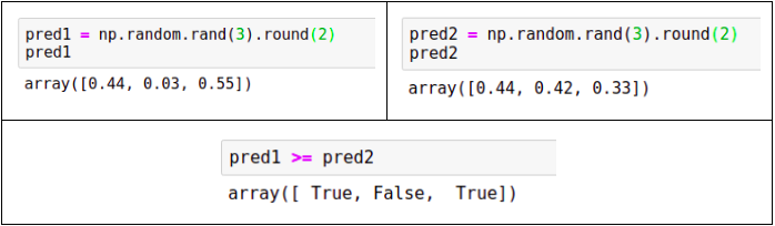
Like with arithmetic operations, we can apply boolean operations on two NumPy arrays of the same shape. Let’s generate two random arrays:
pred1 = np.random.rand(3).round(2)
pred2 = np.random.rand(3).round(2)
The arrays have the following values:
array([0.44, 0.03, 0.55])
array([0.44, 0.42, 0.33])
Now we can use the greater-than-or-equal-to operator (“>=”) to compare the values of these arrays:
pred1 >= pred2
As a result, we get an array with booleans:
array([ True, False, True])
Finally, we can apply logical operations – like logical “and” (“&”) and “or” (“|”) – to boolean NumPy arrays. Let’s again generate two random arrays:
pred1 = np.random.rand(5) >= 0.3
pred2 = np.random.rand(5) >= 0.4
The generated arrays have the following values:
array([ True, False, True])
array([ True, True, False])
Like arithmetical operations, logical operators are also element-wise. For example, to compute the element-wise “and”, we simply use the “&” operator with arrays:
res_and = pred1 & pred2
As a result, we get:
array([ True, False, False])
The logical “or” works in the same way:
res_or = pred1 | pred2
Which creates the following array:
array([ True, True, True])
Summarizing operations
While element-wise operations take in an array and produce an array of the same shape, the summarizing operations take in an array and produce a single number.
For example, we can generate an array and then calculate the sum of all elements:
pred = np.random.rand(3).round(2)
pred_sum = pred.sum()
In this example, pred is
array([0.44, 0.03, 0.55])
Then pred_sum is the sum of all three elements, which is 1.02:
Other summarizing operations include min, mean, max and std:
print('min = %.2f' % pred.min())
print('mean = %.2f' % pred.mean())
print('max = %.2f' % pred.max())
print('std = %.2f' % pred.std())
After running this code, it produces
min = 0.03
mean = 0.34
max = 0.55
std = 0.22
When we have a two-dimensional array, summarizing operations also produce a single number. However, it’s also possible to apply these operations to rows or columns separately.
For example, let’s generate a 4x3 array:
matrix = np.random.rand(4, 3).round(2)
This generates an array:
array([[0.44, 0.03, 0.55],
       [0.44, 0.42, 0.33],
       [0.2 , 0.62, 0.3 ],
       [0.27, 0.62, 0.53]])
When we invoke the max method, it returns a single number:
matrix.max()
The result is “0.62”, which is the maximal number across all elements of the matrix.
If now we want to find the largest number in each row, we can use the max method specifying the axis, along which we apply this operation. When we want to do it for rows, we use axis=1:
matrix.max(axis=1)
As a result, we get an array with four numbers &ndash the largest number in each row:
array([0.55, 0.44, 0.62, 0.62])
Likewise, we can find the largest number in each column. For that, we use axis=0:
matrix.max(axis=0)
This time the result is three numbers &ndash the largest numbers in each column:
array([0.44, 0.62, 0.55])
In NumPy, “axis=1” means applying it to rows and “axis=0” means applying it to columns:

Other operations – sum, min, mean, std and many others – also can take axis as an argument. For example, we can easily calculate the sum of elements of every row:
matrix.sum(axis=1)
When executing it, we get four numbers:
array([1.02, 1.19, 1.12, 1.42])
Sorting
Often we need to sort elements of an array. Let’s see how to do it in NumPy. First, let’s generate a one-dimensional array with four elements:
pred = np.random.rand(4).round(2)
The array we generate contains the following elements:
array([0.44, 0.03, 0.55, 0.44])
To create a sorted copy of the array, use np.sort:
np.sort(pred)
It returns an array with all the elements sorted:
array([0.03, 0.44, 0.44, 0.55])
Since it creates a copy and sorts it, the original array pred remains unchanged.
If we want to sort the elements of the array in-place without creating another array, we invoke the method sort on the array itself:
pred.sort()
Now the array pred becomes sorted.
When it comes to sorting, there’s another useful thing: argsort. Instead of sorting an array, it returns the indices of the array in the sorted order:
idx = pred.argsort()
Now the array idx contains indices in the sorted order:
array([1, 0, 3, 2])
Now we can use the array idx with indexes to get the original array in the sorted order:
pred[idx]
As we see, it’s indeed sorted:
array([0.03, 0.44, 0.44, 0.55])
So, the function sort sorts the array, while argsort produces an array of indices that sort the array:

Reshaping and combining
Each NumPy array has a shape, which specifies its size. For a one-dimensional array, it’s the length of the array, and for a two-dimensional array, it’s the number of rows and columns. We already know that we can access the shape of an array by using the shape property.
rng = np.arange(12)
rng.shape
The shape of rng is “(12,)”, which means that it’s a one-dimensional array of length 12. Since we used np.arange to create the array, it contains the numbers from 0 till 11 (inclusive):
array([ 0, 1, 2, 3, 4, 5, 6, 7, 8, 9, 10, 11])
It’s possible to change the shape of an array from one-dimensional to two-dimensional. We use the reshape method for that:
rng.reshape(4, 3)
As a result, we get a matrix with 4 rows and 3 columns:
array([[ 0,  1,  2],
       [ 3,  4,  5],
       [ 6,  7,  8],
       [ 9, 10, 11]])
The reshaping worked because it was possible to rearrange 12 original elements into 4 rows with 3 columns. In other words, the total number of elements didn’t change. However, if we attempt to reshape it to “(4, 4)”, it won’t let us:
rng.reshape(4, 4)
When we do it, NumPy raises a ValueError:
---------------------------------------------------------------------------
ValueError                                Traceback (most recent call last)
<ipython-input-176-880fb98fa9c8> in <module>
----> 1 rng.reshape(4, 4)

ValueError: cannot reshape array of size 12 into shape (4,4)
Sometimes we need to create a new NumPy array by putting multiple arrays together. Let’s see how to do it.
First, we create two arrays, which we’ll use for illustration:
vec = np.arange(3)
mat = np.arange(6).reshape(3, 2)
The first one, vec, is a one-dimensional array with three elements:
array([0, 1, 2])
The second one, mat, is a two-dimensional one with three rows and two columns:
array([[0, 1],
       [2, 3],
       [4, 5]])
The simplest way to combine two NumPy arrays is using the np.concatenate function:
np.concatenate([vec, vec])
It takes in a list of one-dimensional arrays and combines them into one larger one-dimensional array. In our case, we pass vec two times, so as a result, we have an array of length six:
array([0, 1, 2, 0, 1, 2])
We can achieve the same result using np.hstack, which is short for “horizontal stack”:
np.hstack([vec, vec])
It again takes a list of arrays and stacks them horizontally, producing a larger array:
array([0, 1, 2, 0, 1, 2])
We can also apply np.hstack to two-dimensional arrays:
np.hstack([mat, mat])
The result is another matrix where the original matrices are stacked horizontally – by columns:
array([[0, 1, 0, 1],
       [2, 3, 2, 3],
       [4, 5, 4, 5]])
However, in case of two-dimensional arrays, np.concatenate works different from np.hstack:
np.concatenate([mat, mat])
When we apply np.concatenate to matrices, it stacks then vertically, not horizontally, like one-dimensional arrays, creating a new matrix with 6 rows:
array([[0, 1],
       [2, 3],
       [4, 5],
       [0, 1],
       [2, 3],
       [4, 5]])
Another useful method for combining NumPy arrays is np.column_stack: it allows us to stack vectors and matrices together. For example, suppose we want to add an extra column to our matrix. For that we simply pass a list that contains the vector, and then the matrix:
np.column_stack([vec, mat])
As a result, we have a new matrix, where vec becomes the first column, and the rest of the mat goes after it:
array([[0, 0, 1],
       [1, 2, 3],
       [2, 4, 5]])
We can apply np.column_stack to two vectors:
np.column_stack([vec, vec])
This produces a two-column matrix as a result:
array([[0, 0],
       [1, 1],
       [2, 2]])
Like with np.hstack, that stacks arrays horizontally, there’s np.vstack that stacks arrays vertically:
np.vstack([vec, vec])
When we vertically stack two vectors, we get a matrix with two rows:
array([[0, 1, 2],
       [0, 1, 2]])
We can also stack two matrices vertically:
np.vstack([mat, mat])
The result is the same as np.concatenate([mat, mat]): we get a new matrix with six rows:
array([[0, 1],
       [2, 3],
       [4, 5],
       [0, 1],
       [2, 3],
       [4, 5]])
The np.vstack function can also stack together vectors and matrices, in effect creating a matrix with new rows:
np.vstack([vec, mat.T])
When we do it, vec becomes the first row in the new matrix:
array([[0, 1, 2],
       [0, 2, 4],
       [1, 3, 5]])
In this code we used the T property of mat. This is a matrix transposition operation, which changes rows of a matrix with columns:
mat.T
Originally, mat has the following data:
array([[0, 1],
       [2, 3],
       [4, 5]])
After transposition, what was a column becomes a row:
array([[0, 2, 4],
       [1, 3, 5]])
Slicing and filtering
Like with Python lists, we can also use slicing for accessing a part of a NumPy array. For example, suppose we have a 5x3 matrix:
mat = np.arange(15).reshape(5, 3)
This matrix has 5 rows and 3 columns:
array([[ 0,  1,  2],
       [ 3,  4,  5],
       [ 6,  7,  8],
       [ 9, 10, 11],
       [12, 13, 14]])
We can access parts of this matrix by using slicing. For example, we can get the first three rows using the range operator (“:”):
mat[:3]
It returns rows indexed by 0, 1 and 2 (3 is not included):
array([[0, 1, 2],
       [3, 4, 5],
       [6, 7, 8]])
If we only need rows 1 and 2, we specify both the beginning and the end of the range:
mat[1:3]
This gives us the rows we need:
array([[3, 4, 5],
       [6, 7, 8]])
Like with rows, we can select only some columns, for example, the first two columns:
mat[:, :2]
Here we have two ranges:
- The first one is simply a colon (“:”) with no start and end, which means “include all rows”
- The second one is a range that includes columns 0 and 1 (2 not included).
So as a result, we get:
array([[ 0,  1],
       [ 3,  4],
       [ 6,  7],
       [ 9, 10],
       [12, 13]])
Of course, we can combine both and select any matrix part we want:
mat[1:3, :2]
This gives us rows 1 and 2 and columns 0 and 1:
array([[3, 4],
       [6, 7]])
If we don’t need a range, but rather some specific rows or columns, we can simply provide a list of indices:
mat[[3, 0, 1]]
This gives us three rows indexed at 3, 0 and 1:
array([[ 9, 10, 11],
       [ 0,  1,  2],
       [ 3,  4,  5]])
Instead of individual indices, it’s possible to use a binary mask to specify which rows to select. For example, suppose we want to choose rows where the first element of a row is an odd number.
To check if the first element is odd, we need to do the following:
- Select the first column of the matrix
- Apply the mod 2 operation (“%”) to all the elements to compute the remainder of the division by 2
- If the remainder is 1, then the number is odd, if 0 – the number is even
This translates to the following NumPy expression:
mat[:, 0] % 2 == 1
At the end it produces an array with booleans:
array([False, True, False, True, False])
We see that the expression is True for rows 1 and 3 and it’s False for rows 0, 2 and 5.
Now we can use this expression to select only rows where the expression is True:
mat[mat[:, 0] % 2 == 1]
This gives us a matrix with only two rows: rows 1 and 3:
array([[ 3,  4,  5],
       [ 9, 10, 11]])
Summary
- The NumPy array is the basic data structure in NumPy. There are one-dimensional and two-dimensional NumPy arrays.
- Arithmetical operations (addition, subtraction, multiplication, division) are applied element-wise in NumPy. These are vectorized operations: they don’t require explicit loops. Also, they are implemented in optimized native code and therefore very fast.
- Summarizing NumPy operations include
max,min,meanandsumand when applied to an array, they produce a single number. For two-dimensional arrays it’s possible to perform these operations separately to each row or column of a matrix by specifying the axis along which the operation should be applied.